Estimating the Stability of Psychological Dimensions via Bootstrap Exploratory Graph Analysis: A Monte Carlo Simulation and Tutorial

Abstract

Exploratory Graph Analysis (EGA) has emerged as a popular approach for estimating the dimensionality of multivariate data using psychometric networks. Sampling variability, however, has made reproducibility and generalizability a key issue in network psychometrics. To address this issue, we have developed a novel bootstrap approach called Bootstrap Exploratory Graph Analysis (bootEGA). bootEGA generates a sampling distribution of EGA results where several statistics can be computed. Descriptive statistics (median, standard error, and dimension frequency) provide researchers with a general sense of the stability of their empirical EGA dimensions. Structural consistency estimates how often dimensions are replicated exactly across the bootstrap replicates. Item stability statistics provide information about whether dimensions are unstable due to misallocation (e.g., item placed in the wrong dimension), multidimensionality (e.g., item belonging to more than one dimension), and item redundancy (e.g., similar semantic content). Using a Monte Carlo simulation, we determine guidelines for acceptable item stability. After, we provide an empirical example that demonstrates how bootEGA can be used to identify structural consistency issues (including a fully reproducible R tutorial). In sum, we demonstrate that bootEGA is a robust approach for identifying the stability and robustness of dimensionality in multivariate data.

1. Introduction

Exploratory Graph Analysis (EGA) [1,2] is a recently developed network psychometrics approach for identifying dimensions in multivariate data using network models. Network models are depicted by nodes (circles), which represent variables, and edges (lines), which represent the relation (e.g., partial correlation) between two nodes. Communities or clusters of nodes represent dimensions in networks. EGA is based on the estimation of a network followed by the application of a community detection algorithm [3].

Although EGA has become a popular approach for dimensionality assessment in the psychometric network literature, there remain lingering questions related to the stability of its results. The reproducibility of psychometric networks is an area that has received a lot of attention in recent years [4,5,6,7]. Variability, whether related to random sampling or parameter estimation, can have downstream effects on analyses that are applied to a network such as centrality measures (i.e., measures that quantify the relative position of a node in the network) and community detection algorithms. For the latter, variability may lead to dimensional structures that do not generalize to other samples, potentially leading to inconsistencies in the number and content of the communities in the network. The goal of the present paper is to introduce a novel bootstrap approach that provides information about the stability of EGA’s results.

2. Exploratory Graph Analysis

The most commonly applied network estimation method in the literature is the graphical least absolute shrinkage and selection operator (GLASSO) [8,9]. The GLASSO estimates a Gaussian Graphical Model (GGM) [10], where edges are the partial correlation between two nodes given all other nodes in the network. The GLASSO penalizes and shrinks coefficients (with small coefficients going to zero) to provide more parsimonious results and lower the potential for spurious relations.

The GLASSO uses a regularization technique called the least absolute shrinkage and selection operator (LASSO) [11]. The LASSO has a hyperparameter $\lambda$, which controls the sparsity of the network. Lower values of $\lambda$ remove fewer edges, increasing the possibility of including spurious correlations, while larger values of $\lambda$ remove more edges, increasing the possibility of removing relevant edges. When $\lambda =0$, the estimates are equal to the ordinary least squares solution for the partial correlation matrix.

A common approach in the network psychometrics literature is to compute models across several values of $\lambda$ (usually 100) and select the model that minimizes the extended Bayesian information criterion (EBIC) [12,13]. The EBIC has a hyperparameter ($\gamma$), which controls how much it prefers simpler models (i.e., models with fewer edges) [14]. Larger $\gamma$ values lead to simpler models, while smaller $\gamma$ values lead to denser models. When $\gamma =0$, the EBIC is equal to the Bayesian information criterion. The EGA approach starts with $\gamma =0.50$ and lowers $\gamma$ by 0.25 if there are any unconnected nodes in the network (i.e., if a node does not have an edge to any other nodes). If $\gamma$ reaches zero, then the network is used regardless of whether there are unconnected nodes in the networks.

More recently, the triangulated maximally filtered graph (TMFG) [15] has been applied as an alternative network estimation method in EGA [2,16]. The TMFG method uses a structural constraint that limits the number of zero-order correlations included in the network ($3n-6$; where n is the number of variables). The TMFG algorithm begins by identifying four variables that have the largest sum of correlations to all other variables. Then, it iteratively adds each variable with the largest sum of three correlations to nodes already in the network until all variables have been added to the network. The end result is a network of 3- and 4-node cliques (i.e., a set of connected nodes), which form the constituent elements of an emergent hierarchy in the network [17].

In psychometric networks, clusters (or sets of many connected nodes) often emerge, forming distinct communities or sub-networks of related nodes. To estimate communities, community detection algorithms can be applied [3,18,19]. The most commonly applied algorithm used in EGA is the Walktrap community detection algorithm. The Walktrap algorithm estimates the number and content of a network’s communities using “random walks” over the network [20]. These random walks iteratively traverse over neighboring edges, with larger edge weights (i.e., partial correlations) being more probable paths of travel. Each node is repeatedly used as a starting point where steps—a jump from one node over an edge to another—are taken away from that node, forming a community boundary. A node’s community is then determined by its proportion of many densely connected edges to few, sparsely connected edges (commonly optimized by a statistic known as modularity) [21]. The algorithm is deterministic, meaning the number and variable content of the communities are estimated without the researcher’s direction. These communities are shown to be consistent with latent factors of factor models [1]. For more details about all network estimation methods and the Walktrap algorithm, see Section 9.

3. EGA Compared to Factor Analytic Methods

There have been several simulation studies comparing EGA to factor analytic methods. In Golino and Epskamp’s [1] seminal simulation, EGA was compared against several commonly used factor analytic methods, including the Kaiser–Guttman rule (eigenvalues > 1) [22,23], minimum average partial procedure [24], and parallel analysis (PA) [25]. Overall, EGA and PA with principal axis factoring (PAF) performed the best of the methods with 96% and 97% overall accuracy (respectively). EGA tended to perform better when there were fewer variables per factor (5) and moderate-to-high correlations between factors (0.50 and 0.70), while PA tended to perform better when there were more variables per factor (10) and moderate-to-high correlations between factors.

The second simulation expanded on the first by adding the TMFG network estimation method and PA with principal component analysis (PCA), estimating unidimensional structures, manipulating skew, factor loadings, and data categories (continuous and dichotomous variables) [2]. Once again, EGA with GLASSO and PA with PCA and PAF had the best overall accuracy (88%, 82%, and 83%, respectively). EGA with TMFG was in the middle of the pack with an overall accuracy of 73%. The PA methods tended to perform better when there were more variables per factor (8 and 12), while EGA with GLASSO tended to perform better when there were fewer variables per factor (3 and 4). EGA with TMFG performed best when there were 4 and 8 variables per factor. EGA with GLASSO (96%) and PA with PCA (100%) performed better than PA with PAF when the data were unidimensional, while EGA with GLASSO (84%) and PA with PAF (83%) performed better than PA with PCA when the data were multidimensional. EGA with TMFG trailed behind all three with 79% accuracy for unidimensional structures and 73% accuracy for multidimensional structures.

A more recent simulation assessed different community detection algorithms (including the Walktrap) combined with EGA with GLASSO compared to the PA methods using continuous and polytomous (5-point Likert scale) data [18]. In this study, factor loadings were drawn randomly from a uniform distribution between 0.40 and 0.70. The Louvain (90%) [26], Fast-greedy (89%) [27], and Walktrap (88%) [20] algorithms had comparable overall accuracy with PA with PCA (88%) and PAF (85%). The number of factors had the biggest effects on performance, particularly when there were more factors (e.g., 4), where the Louvain and Fast-greedy algorithms were comparable to PA with PAF (around 90%), but the Walktrap was much less accurate (around 80%). In sum, EGA with GLASSO performs comparably to common factor analytic methods such as parallel analysis. Despite evidence of EGA’s effectiveness, there has yet to be an investigation into the stability of its results.

4. Bootstrap Approach

To address this issue, we introduce a novel approach called Bootstrap Exploratory Graph Analysis (bootEGA) to estimate the stability of dimensions identified by EGA. This approach allows for the consistency of dimensions and items to be evaluated across bootstrapped EGA results, providing information about whether the data are consistently organized in coherent dimensions or fluctuate between dimensional configurations. On the one hand, the number of dimensions identified may vary depending on the size of the sample or the sample being measured (e.g., measurement (in)variance). On the other hand, the number of dimensions might be consistent across samples, but some items may be identified in one dimension in one sample and in another dimension in a different sample. Even still, some sets of items may be forming completely separate dimensions.

Using a bootstrap approach, the bootEGA algorithm uses one of two data generation approaches: parametric or resampling (non-parametric). The parametric procedure begins by estimating the empirical correlation matrix. This correlation matrix is then used as the covariance matrix to generate data from a multivariate normal distribution. The resampling or non-parametric procedure is implemented by resampling with a replacement from the empirical dataset. The parametric procedure should be preferred when the underlying data are expected to follow a multivariate normal distribution. The resampling procedure should be preferred when the underlying distribution is unknown or non-normal. Regardless of procedure, the same number of cases as the original dataset is used to generate or resample data. For each replicate sample, EGA is applied, resulting in a sampling distribution of EGA results. This process continues iteratively until the desired number of samples is achieved (e.g., 500).

4.1. Descriptive Statistics

From this sampling distribution, several descriptive statistics are obtained. The median number of dimensions estimated from the replicate samples is computed. The standard deviation of the number of dimensions is used as the standard error. A normal approximation confidence interval is computed by using this standard error and multiplying it by the 2.5 and 97.5 percentile of a t-distribution with iterations minus one degree of freedom [28]. Finally, a percentile bootstrap confidence interval is computed using the same percentiles in the bootstrap quantiles [29]. In addition, a median (or typical) network structure is estimated by computing the median value of each edge across the replicate networks, resulting in a single network. Such a network represents the “typical” network structure of the sampling distribution. The community detection algorithm was then applied, resulting in dimensions that would be expected for a typical network from the EGA sampling distribution.

4.2. Dimension and Item Stability

Because EGA assigns variables to dimensions, additional metrics related to the stability of dimensions and items across bootstrap replicates can be computed. bootEGA evaluates the stability of dimensions using a measure called structural consistency. We define structural consistency as the proportion of times that each empirically derived dimension (i.e., the result from the initial EGA) that was exactly recovered (i.e., identical item composition) from the replicate bootstrap samples was computed. Below, we provide an example of how structural consistency is computed.

Let w be the placement of items in the empirical EGA communities:

$$w=\{1,1,1,2,2,2,3,3,3,...,j,j,j\},$$

where values j denote dimensions (e.g., 1 denotes dimension 1). Let $b^i$ be the bootstrap placement of items for the $i\mathrm{th}$ iteration of bootEGA. For example, the first iteration:}

$$b^1=\{1,1,1,2,2,3,3,3,3,...,j,j,j\}.$$

If all elements corresponding to the $j\mathrm{th}$ dimension of the empirical item placement and the bootstrap iteration placement match, then the dimension is given a value of 1 for the iteration; otherwise 0. For example, the first three elements of the empirical item placement w correspond to dimension 1. The first three elements of $b^1$ are also all 1 and therefore match (1). The next three elements of the empirical item placement w correspond to dimension 2. For $b^1$, these elements are $\{2,2,3\}$ and therefore do not match (0). Finally, the last three elements of the empirical item placement w correspond to dimension 3. For $b^1$, these elements are all 3 and therefore match (1).

Let $d_j^i$ be a vector storing the values of whether the bootstrap placement of items match the empirical placement of items for dimension j and iteration i. For the example above, $d^1=\{1,0,1\}$. The structural consistency of each dimension is then defined as:

$$s_j=\frac{{\sum }_i^n{d}_j^i}{n},$$

where n is the number of iterations and $s_j$ is the structural consistency of dimension j.

Substantively, we interpret structural consistency as the extent to which a dimension is interrelated (internal consistency) and homogeneous (test homogeneity) in the presence of other related dimensions [30]. Such a measure provides an alternative yet complementary approach to internal consistency measures in the factor analytic framework.

A complementary measure to structural consistency is item stability. Item stability quantifies the robustness of each item’s placement within each empirically derived dimension. Item stability is estimated by computing the proportion of times each item is placed in each dimension. This metric provides information about which items are leading to structural consistency (replicating often in their empirically derived dimension) or inconsistency (replicating often in other dimensions).

One obstacle for computing item stability is that item placement is not always consistent with the empirical placement. As demonstrated in $b^1$ above, dimension 2 was only two elements and dimension 3 was four elements relative to both having three elements each in the empirical item placement. Below are several examples that can be compared with w:

$$\begin{array}{c}\hfill w=\{1,1,1,2,2,2,3,3,3\}\\ \hfill b^1=\{1,1,1,2,2,3,3,3,3\}\\ \hfill b^2=\{3,3,3,1,1,1,2,2,2\}\\ \hfill b^3=\{1,1,1,1,1,2,2,2,2\}\\ \hfill b^4=\{3,3,2,2,2,1,1,1,1\}.\end{array}$$

(1)

Starting with $b^2$, the composition of w and $b^2$ are the same, but their number assignments differ. This is a common occurrence as EGA does not always assign dimension 1 to the label number 1 as it is in w. In this example, the solution is obvious: 3 becomes 1, 1 becomes 2, and 2 becomes 3.

For $b^3$, the categorization is not immediately clear. First, there are only two dimension labels (1 and 2). Second, the elements corresponding to the second empirical dimension overlap in $b^3$: $\{1,1,2\}$. To circumvent these issues, the item stability algorithm follows several steps to produce what we call “homogenized” item placements. First, the Adjusted Rand Index (ARI) [31] is computed between each dimension’s elements of the item placement in the bootstrap iteration ($b^3$) and the corresponding elements for the empirical item placements (w). The ARI is computed using the following formula:

$$ARI=\frac{\left(\genfrac{}{}{0pt}{}{N}{2}\right)(a+d)-[(a+b)(a+c)+(c+d)(b+d)]}{{\left(\genfrac{}{}{0pt}{}{N}{2}\right)}^2-[(a+b)(a+c)+(c+d)(b+d)]}$$

where a is the count of items placed into the same bootstrap and empirical community and d is the count of items that are in different communities of both the bootstrap and empirical communities. Both b and c count the wrong placement of nodes between the bootstrap community and empirical community, respectively.

For dimension 1 of $b^3$ and the corresponding elements in w ($\{1,1,1,2,2\}$), the ARI equals 0.4. For dimension 2 of $b^3$ and the corresponding elements in w ($\{2,3,3,3\}$), the ARI equals 0.5. The next step orders the dimensions based on highest to lowest ARI first. Ties are decided based on the number of items in the respective dimensions from highest to lowest. This ordering ensures that (1) dimensions that correspond closest to the empirically defined dimensions (e.g., w) are handled first and (2) that dimensions that are most intact (i.e., that have more items) are handled prior to equivalent ARI values.

The final step is identifying the mode in which the respective elements of w belong to. For dimension 3 of $b^3$, the mode is 1 and therefore converts all labels of 3 to 1. For dimension 2 of $b^3$, the mode is 3 and therefore converts all labels of 2 to 3. The result is a “homogenized” item placement for $b^3$ of $\{1,1,1,1,1,3,3,3,3\}$. Following these steps for $b^4$, the result is $\{1,1,2,2,2,3,3,3,3\}$. Once all bootstrap item placements have been homogenized with the empirical item placements, then item stability values can be computed. These values are computed by taking the number of times an item is assigned to each dimension and dividing it by the total number of bootstrap iterations.

5. Present Research

In the present paper, we introduce bootEGA to estimate the stability of dimensions identified by EGA. The goal of bootEGA is to provide a tool for assessing whether dimensions and items in a scale are generalizable. Unstable dimensions and items are important for diagnosing psychometric issues that may lead to inappropriate scale interpretations. Items sorting into different dimensions, for example, may be an issue of sample size, hint that the items are multidimensional, or that they are redundant with one another and are forming a minor factor [32,33]. Therefore, an approach that is able to assess the quality of EGA’s results is necessary and would allow researchers to examine how their results would be expected to generalize to other samples. Such an approach would not only lead to more accurate interpretations but also provide researchers with greater insights into the structure of their scales.

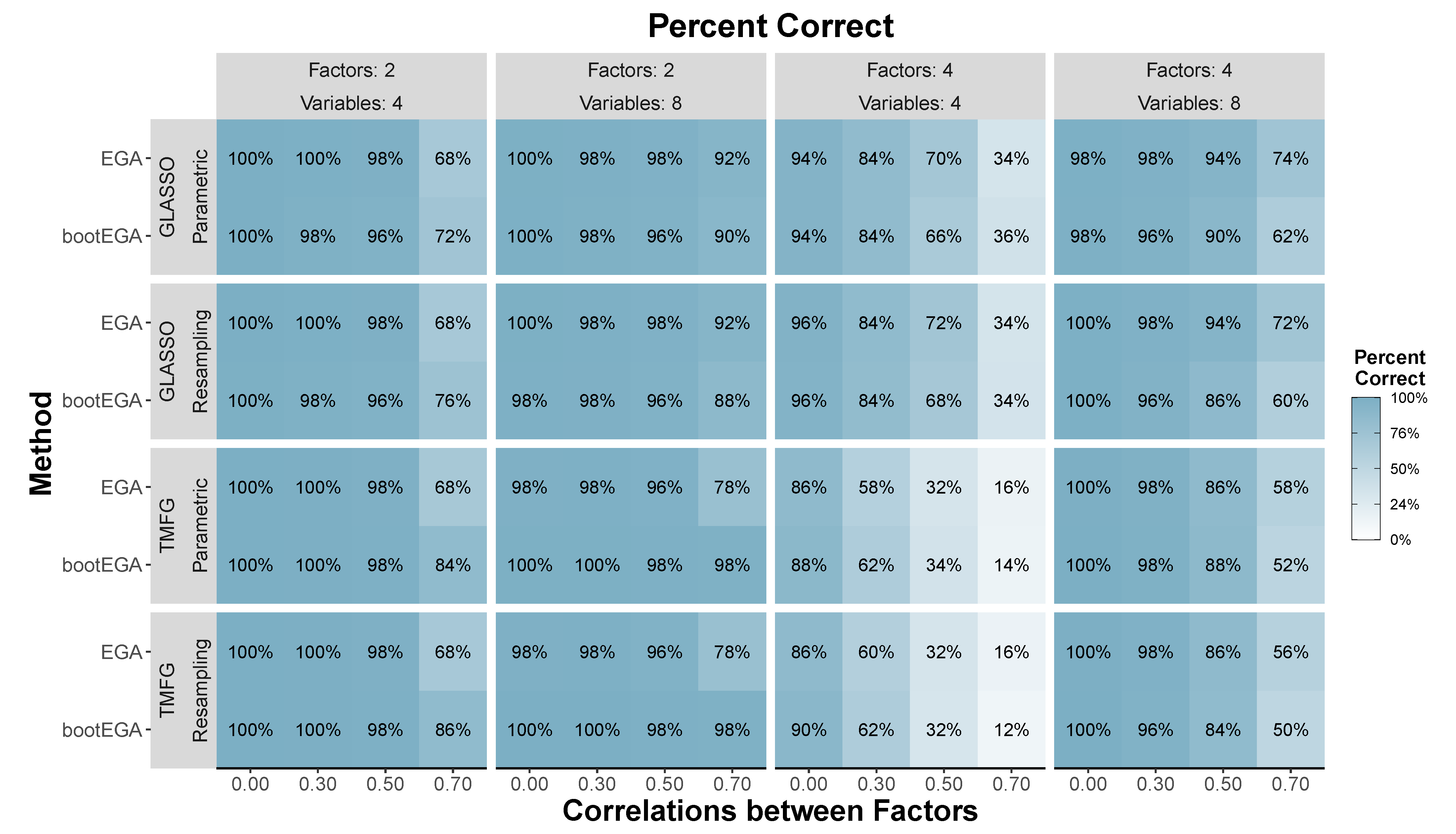
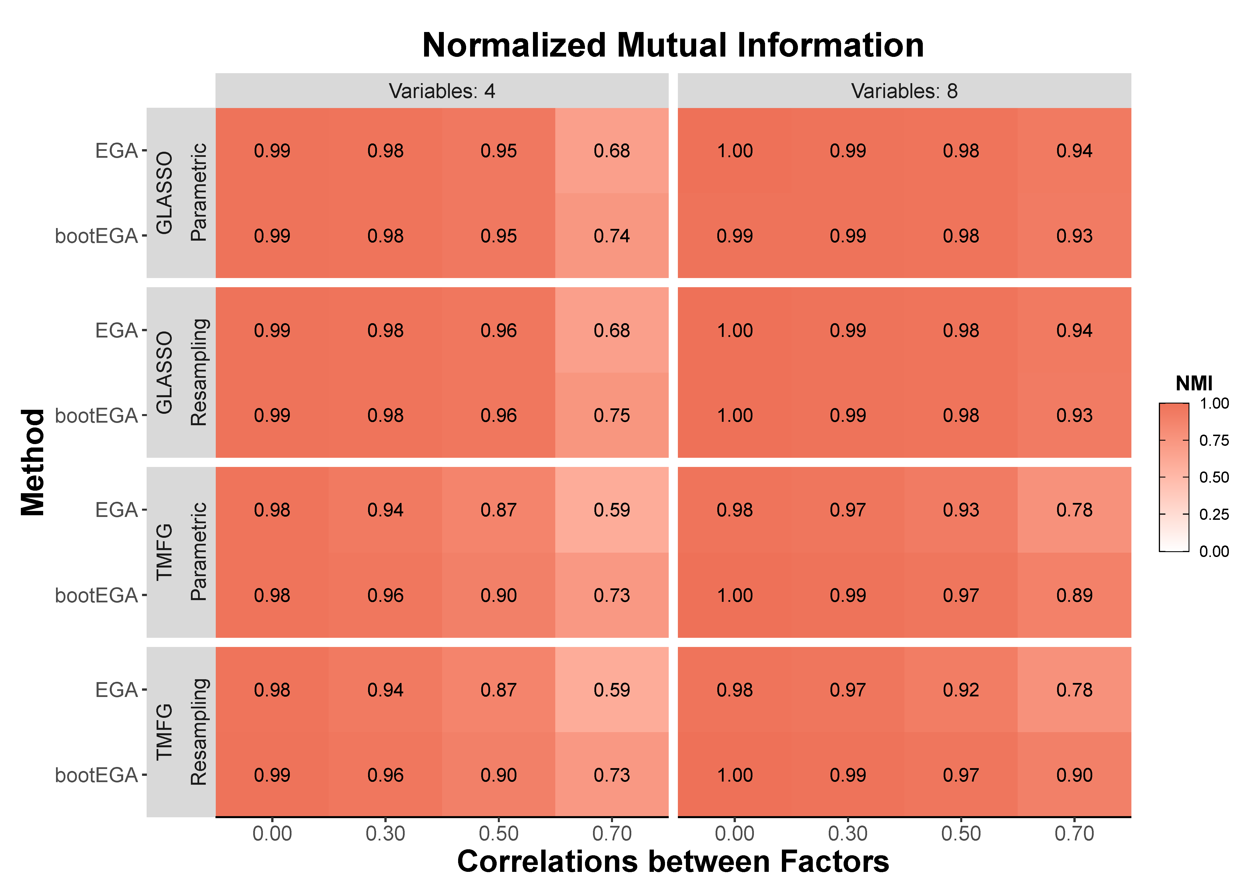
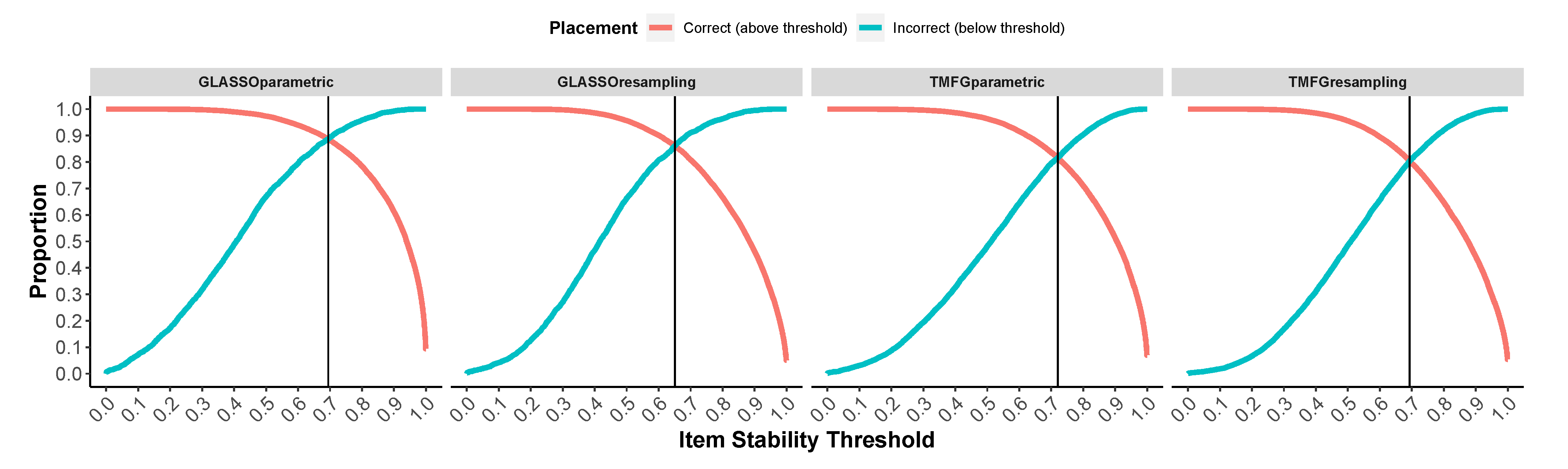
To investigate the validity of the bootEGA approach and item stability analysis, we conducted a large simulation study. In this study, we manipulated sample size (250, 500, and 1000), number of factors (2 and 4), number of variables per factor (4 and 8), correlations between factors (0.00, 0.30, 0.50, and 0.70), and data categories (continuous and polytomous). Importantly, we generated data with cross-loadings and factor loadings that varied randomly between 0.40 and 0.70. We also added skew to the polytomous data ranging from −2 to 2 on 0.5 increments. The first aim was to determine whether the typical structure of bootEGA could improve the accuracy of empirical EGA’s dimensionality accuracy and item placement. The second aim was to determine guidelines for what values of item stability reflect a “stable” item. For this latter aim, we used data from the largest sample size condition only to ensure the robustness of the guidelines we propose.

After, we provide an empirical example to show how to apply and interpret bootEGA output. In the example, we demonstrate that bootEGA can be used to improve the structural integrity of assessment instruments through the identification of problematic items. We show that problematic items can arise because several items are multidimensional (i.e., they replicate in other dimensions and cross-load onto more than one dimension). As part of the empirical example, we provide tutorial code that researchers can apply to their own data. The R code for the simulation, analyses, and example are available on our Open Science Framework repository: https://osf.io/wxdk7/ (accessed on 24 April 2021).

6. Results

6.1. Dimensionality Accuracy

Our first goal was to determine whether the typical bootEGA network structure could improve on the dimensionality accuracy and item placement of the empirical EGA structure. Despite generating both continuous and polytomous data, there was no effect of data categories. Therefore, we collapsed across data categories. The typical structure of bootEGA was comparable to the empirical structure in terms of accuracy. The type of bootstrap did not have a substantial influence on the percent correct (PC; identifying the same number of dimensions as the number of simulated dimensions), with all PCs within a single percent of one another for both the GLASSO and TMFG. Empirical GLASSO was slightly more accurate (87.5%) than bootEGA GLASSO (86.1%), while empirical TMFG was less accurate (79.6%) than bootEGA TMFG (82.2%). There were three main effects that were at least a moderate effect size: number of variables per factor (${\eta }_p^2=0.06$), number of factors (${\eta }_p^2=0.13$), and correlations between factors (${\eta }_p^2=0.18$). There were no interactions between the conditions. Figure 1 breaks these results down by the conditions that had main effects.

These main effects are made clearer by Figure 1: accuracy increased as variables per factor increased, accuracy decreased as the number of factors increased, and accuracy decreased as correlations between factors increased. The worst condition for all methods was when there were four variables per factor and four factors. In this condition, GLASSO remained fairly high in accuracy (around 70–90%) as correlations between factors increased until large correlations (0.70), where their accuracy dropped by about 40%. In contrast, TMFG had large decreases in accuracy with each increase in correlations between factors (around 20%). The differences between bootEGA and EGA were subtle. bootEGA tended to increase accuracy as correlations between factors increased. This pattern was particularly true for the TMFG method, suggesting that it benefits from obtaining a typical structure more than the GLASSO method.

It is noteworthy that there was no effect of sample size given that the number of cases tend to affect most methods [34]. Digging into our results, there was an apparent ceiling effect across conditions that might have limited the effect of sample size. Specifically, there only appeared to be a performance difference when there were less favorable conditions: few variables (4) and large correlations between factors (0.70).

Similar to accuracy, there was not an effect of data categories with item placement (normalized mutual information; NMI; see Section 9 for mathematical notation). Further, the typical structure of bootEGA was comparable to the empirical EGA. The type of bootstrap also did not have an effect on item placement. bootEGA (0.944) and empirical (0.941) EGA were comparable for GLASSO, but bootEGA (0.928) was higher than empirical (0.881) for TMFG. There was a moderate interaction between the number of variables and correlations between factors (${\eta }_p^2=0.07$).

Figure 2 shows that this interaction was mainly driven by large correlations between factors (0.70). There was a stark drop in NMI (around 0.20) from eight variables per factor to four variables per factor with these large correlations between factors. For both GLASSO and TMFG, bootEGA improved item placement in these conditions relative to empirical EGA. For all other conditions, bootEGA was comparable with empirical EGA. In sum, bootEGA provided comparable accuracy when estimating the number of dimensions and provided comparable or better item placement of items within those dimensions. TMFG particularly benefited from bootEGA.

6.2. Item Stability

To derive item stability guidelines, we collapsed across all conditions to evaluate the value at which the proportion of times an item replicating in a factor could be considered “stable” across bootstraps. To achieve this, we identified which simulated samples did not have NMI values equal to one (i.e., perfect item assignment) for empirical EGA. Item stability or the proportion of times an item replicated in the simulated dimension was then computed. We then separated items that were assigned correctly and incorrectly. Using each assignment’s item stability values, we then computed the proportion of item stability values that were above or below an incremental threshold (from 0 to 1 on 0.001 increments).

For the correctly assigned items, we computed the proportion of item stability values that were at or above the threshold. For the incorrectly assigned items, we computed the proportion of item stability values that were below the threshold. This approach provided inference into where items could be considered stable. Specifically, the item stability value where the correctly and incorrectly assigned proportion lines crossed is the optimal threshold for maximizing items that are identified as being correctly assigned as being in the correct or incorrect population factor. The plots for each network estimation method and bootstrap type combination are presented in Figure 3.

For each plot, the proportion of values that maximized the the correct and incorrect placements differed slightly for the GLASSO and TMFG methods (see vertical black lines in Figure 3). Values higher or lower than these optimal points suggest a bias towards favoring identification of correctly identifying items that are correctly placed (or correctly identifying items that are incorrectly placed). Therefore, these points represent the optimal balance in the trade-off of false positives and negatives in determining whether an item is stable or unstable. For the GLASSO method, these optimal points were at item stability values of 0.695 and 0.651 for parametric and resampling bootstraps, respectively. For the TMFG method, these optimal points were at item stability values of 0.721 and 0.694 for parametric and resampling bootstraps, respectively. These results suggest that values around 0.65–0.75 are about when variables start to become less stable.

7. Applied Example: Broad Autism Phenotype Questionnaire

To demonstrate how the bootEGA approach can be applied to investigate the stability of the structure of empirical data, we used data from the Simons Simplex Collection (SSC), a core project and resource of the Simons Foundation Autism Research Initiative that established a permanent repository of genetic and phenotypic samples from 2600 simplex families. Each family has one child affected with an autism spectrum disorder with unaffected parents and siblings. Here, we used Broad Autism Phenotype Questionnaire (BAPQ) [35] data completed by mothers and fathers (n = 5659) of children with an autism spectrum disorder. Before applying with the dataset, the reader will need to install and load the latest EGAnet package:

After installing EGAnet, the reader should install, authenticate, download, and load data from our OSF:

With the correlation matrix of BAPQ loaded, EGA can be applied. Below, we use the default EGA approach, which is to use the GLASSO network estimation method with the Walktrap community detection algorithm:

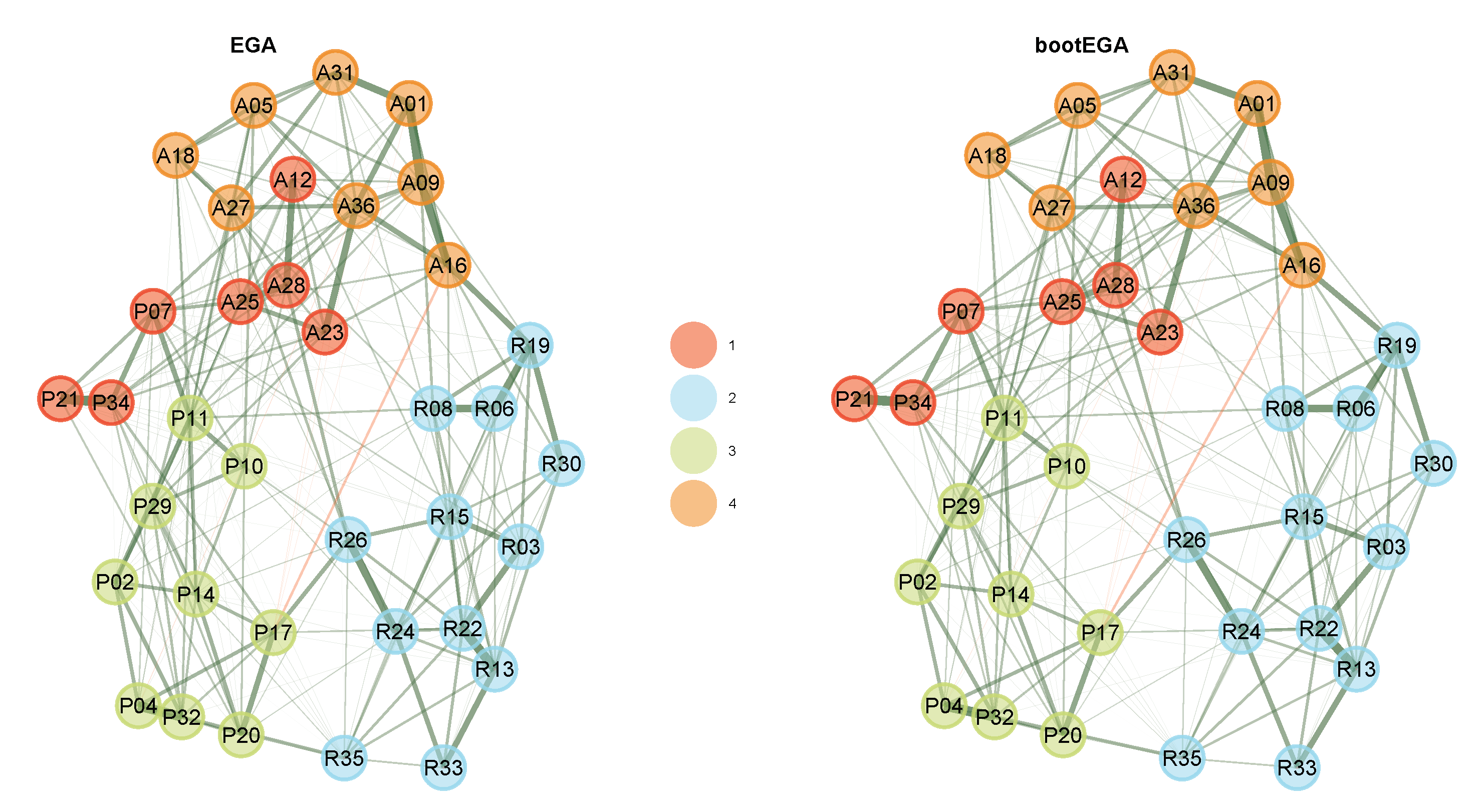
Exploratory Graph Analysis with the GLASSO network estimation method and the Walktrap community detection algorithm estimated four factors (Figure 4), representing the theoretical factors. Dimension 2 is consistent with the rigid dimension (R3, R6, R8, R13, R15, R19, R22, R24, R26, R30, R33, R35). Dimension 3 is consistent with the pragmatic language dimension (P2, P4, P10, P11, P14, P17, P20, P21, P29, P32, P34). Dimension 4 is consistent with the aloof dimension (A1, A5, A9, A16, A18, A27, A31, A36). Dimension 1, however, represents a mix of the aloof (A12, A23, A25, A28) and pragmatic language (P7, P21, P34) dimensions.

Curiously, these items all reflect difficulty in social interactions with other people: A12 (“People find it easy to approach me”), A23 (“I am good at making small talk”), A25 (“I feel like I am really connecting with other people”), A28 (“I am warm and friendly in my interactions with others”), P07 (“I am ‘in-tune’ with the other person during conversation”), P21 (“I can tell when someone is not interested in what I am saying”) and P34 (“I can tell when it is time to change topics in conversation”). While we may be interested in interpreting this dimension, it is important to know whether these dimensions are stable and likely to reproduce in other samples. To achieve so, we can apply bootEGA for 500 iterations:

Because our dataset is a correlation matrix, the resampling (non-parametric) bootstrap option is not available. Recall that the resampling requires shuffling cases with replacement. Proceeding with the parametric bootstrap, we find that the median network structure depicted in Figure 4 has four dimensions, similar to the empirical EGA. To evaluate the stability of these dimensions, we can start first by checking the descriptive statistics (

Table 1. Descriptive statistics of BAPQ dimensions across all bootstrap replicate samples.

n.Boots	median.dim	SE.dim	CI.dim	Lower.CI	Upper.CI	Lower.Quantile	Upper.Quantile
500	4	0.458	0.9	3.1	4.9	3	4

):

Here, we can see that the median is four dimensions, mirroring the empirical EGA with a relatively narrow confidence interval (CI 95% [3.10, 4.90]). To get a better idea of this distribution, we can look at the frequency of each dimension solution (

Table 2. Frequency of BAPQ dimensions across all bootstrap replicate samples.

# of Factors	Frequency
3	0.298
4	0.702

):

With the frequencies, four dimensions were found 70.20% of the time or 351 of 500 bootstrap replicates while three dimensions were found 29.80% of the time or 149 of 500 bootstrap replicates. These results seem to suggest that the four dimension solution might be unstable. To get a better understanding of what dimensions in particular are unstable, we can compute structural consistency or how often the empirical EGA dimension is exactly replicated (identical item assignments) across the bootstrap replicates (

Table 3. Dimension stability of BAPQ items across all bootstrap replicate samples.

	Dimension Stability
1	0.574
2	1.000
3	0.930
4	1.000

) [30]:

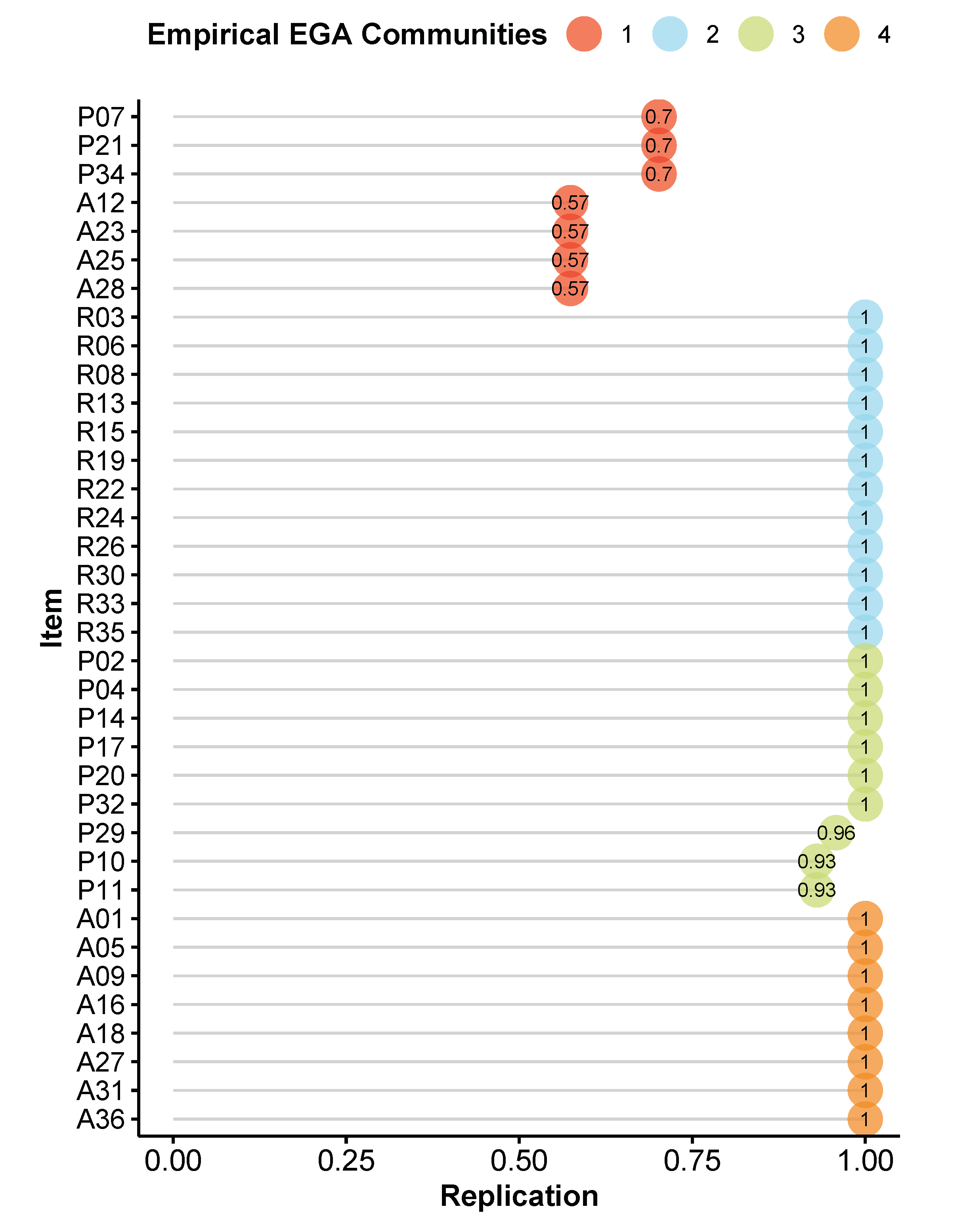
The structural consistency result shows that dimension 1, which represented the difficulty with social interactions, is very unstable. Indeed, this is confirmed when looking at the item stability values in the empirical dimensions (Figure 5). All items from dimension 1 are at or below the range of 0.65–0.75, where they can be considered unstable.

Table 4. Item stability of BAPQ items across all bootstrap replicate samples.

	1	2	3	4
P07	0.702		0.298
P21	0.702		0.298
P34	0.702		0.298
A12	0.574			0.426
A23	0.574			0.426
A25	0.574			0.426
A28	0.574			0.426
R03		1
R06		1
R08		1
R13		1
R15		1
R19		1
R22		1
R24		1
R26		1
R30		1
R33		1
R35		1
P02			1
P04			1
P14			1
P17			1
P20			1
P32			1
P29	0.042		0.958
P10	0.07		0.93
P11	0.07		0.93
A01				1
A05				1
A09				1
A16				1
A18				1
A27				1
A31				1
A36				1

shows how the item stability values across each dimension in the replicate bootstrap samples (values of zero have been removed to facilitate interpretability). To probe this instability further, we can look at how these items are replicating across all bootstrap dimensions with the following code:

Table 4 displays the item stability values across each dimension in the replicate bootstrap samples. From this table, it is clear that some items are unstable. Items A12, A23, A25, and A28 are sometimes replicating in dimension 4, which was their theoretical dimension of aloof. Items P7, P21, and P34 are sometimes replicating in dimension 3, which was the theoretical dimension of pragmatic language.

These results suggest that although these items are associated with their theoretical dimension, they share enough conceptual similarity that they form a separate dimension. These unstable items are clearly causing problems with the consistency of the dimensions of the BAPQ, which are likely due to their multidimensional features—that is, sharing an underlying difficulty with social interactions. To verify this, we looked at the average network loadings of these items across the bootstraps (example code: bapq.dimstab$item.stability$item.stability$mean.loadings;

Table 5. Average network loadings of unstable BAPQ items across all bootstrap replicate samples.

	1	2	3	4
P7	0.21	0.02	0.12	0.05
P21	0.21	0.01	0.06	0.01
P34	0.30	0.01	0.13	0.02
A12	0.18	0.02	0.02	0.09
A23	0.15	0.00	0.06	0.15
A25	0.23	0.01	0.06	0.15
A28	0.22	0.03	0.03	0.12

Note. Bold values are network loadings greater than or equal to a small effect size (0.15).

).

Based on the average network loadings, there are a couple of items that have cross-loadings worth consideration (≥0.15) [36]: A23 (1 and 4) and A25 (1 and 4). Similarly, items P7 (0.13), A28 (0.13), and P34 (0.12) have a cross-loading approaching the same threshold. These results suggest that these items are indeed multidimensional. To resolve this issue, we can remove these items and reassess the structure of the BAPQ (Figure 6 and Figure 7).

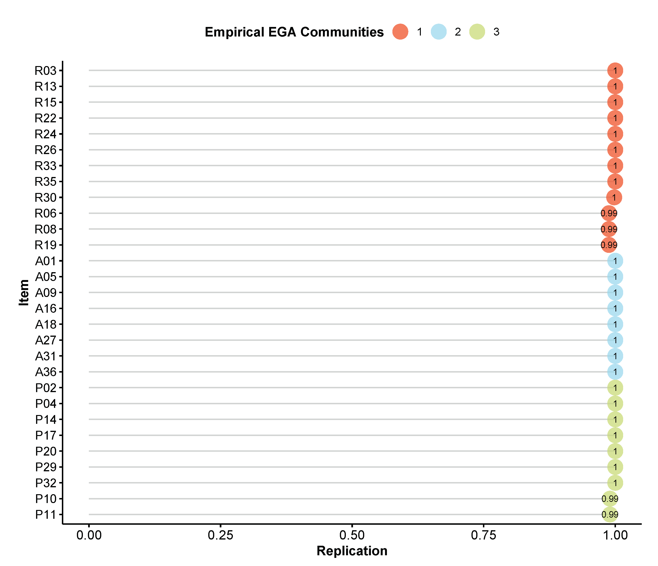
We can follow through with bootEGA to determine how stable the empirical EGA dimensions are after these items are removed. The bootEGA result found that three factors are being estimated in 99% of the bootstrapped samples, and Figure 7 shows that the item stability values are now nearly all 1’s, demonstrating the robustness of the dimensionality solution estimated via EGA. The three factor structure estimated after removing the unstable items are very similar to the original three factor structure proposed by Hurley, Losh, Parlier, Reznick, and Piven [35]. Dimension 1 is composed of items all rigid items (R), dimension 2 of all aloof items (A), and dimension 3 of all pragmatic language items (P).

This example demonstrates that multidimensional items can influence the stability of dimensions and lead to an unstable dimensional structure. Multidimensional items will replicate in two or more dimensions and can potentially be identified by examining the item stability and average network loadings across the bootstraps (e.g., Table 5). Removing these items cleans up the stability of the dimensions, leading to good structural consistency.

8. Discussion

In this paper, we present a novel approach for assessing the stability of dimensions in psychometric networks using EGA. Using a Monte Carlo simulation, we show that the typical structure of bootEGA is comparable to empirical EGA for estimating the number of dimensions but has as good or better item placement. From this simulation, we derived guidelines for acceptable item stability (≥0.70). Finally, we provide an empirical example with an associated R tutorial to demonstrate how to apply and interpret the bootEGA approach. We demonstrated that items with stability values lower than an acceptable value can lead to poor structural consistency. In our example, the poor stability of these items was due to multidimensionality. We show that removing these problematic items led to improved structural consistency.

bootEGA adds another approach to the network psychometric literature for assessing the robustness of network analysis results. Previous work has applied bootstrap approaches to assess the accuracy of estimated edge weights, stability of centrality measures, and test differences between edge weights and centrality values [13]. Our approach expands reserachers’ capabilities to estimate network robustness by enabling them to verify the consistency of dimensions identified by EGA. Importantly, future work will need to examine whether bootEGA provides the same benefits when data have fewer categories than we tested here (i.e., <5). Dichotomous data, for example, may reveal greater differences in performance than the continuous and polytomous (i.e., 5-point Likert scale) data we generated.

As a part of our approach, bootEGA offers diagnostic information about the causes of poor dimensional stability. This has broad implications for scale development. For example, scales are intended to be developed to measure a single attribute. Often, attributes (measured by scales) are multifaceted with separate but related features (measured by subscales). While these features are related, there has yet to be an approach, to our knowledge, to assess the extent to which features remain cohesive (but see, [37]). Such an approach is important for ensuring that each subscale is capturing a distinct feature of the attribute without being confounded by overlap with other features. In simpler language, our approach can help investigate whether the items are hanging together as researchers intend.

Our empirical example examined the BAPQ scale, which has mixed evidence for its internal structures. The BAPQ scale was intended to measure three separate but related factors of the broad autism phenotype. Previous validation studies of the BAPQ factors have shown that many items have sizable cross-loadings between factors [38]. bootEGA’s dimension and item stabilities found that there were seven items belonging to the aloof and pragmatic language factors that were forming their own dimension related to difficulties with social interactions. These items were clarified using network loadings, revealing cross-loadings with considerable size. After removing these items, we identified a three-dimension structure that was structurally consistent and corroborated the theoretical factors. Future work using the BAPQ should strongly consider assessing the stability of the dimensionality of the scale before assuming the theoretical dimensions are being measured as intended.

In summary, bootEGA offers researchers several novel tools for assessing the structural integrity of their scales from the psychometric network perspective. Our approach represents both an advance in network psychometrics as well as constructs validation more generally. For network analysis, researchers can assess the stability of the dimensions of the networks. For the broader construct validation literature, researchers can assess whether the structure of their subscales remain homogeneous (i.e., unidimensional) in a multidimensional context.

9. Materials and Methods

9.1. Data Generation

We generated data from multivariate normal factor models following the same approach as Golino et al. [2]. First, the reproduced population correlation matrix was computed:

$${\mathbf{R}}_{\mathbf{R}}=\mathsf{\Omega }\mathsf{\Phi }{\mathsf{\Omega }}^{\prime },$$

where ${\mathbf{R}}_{\mathbf{R}}$ is the reproduced population correlation matrix, $\mathsf{\Omega }$ is the k (variables) × r (factors) factor loading matrix (the traditional notation for factor loadings matrix is $\Lambda$; however, to avoid confusion with the GLASSO’s lambda parameter ($\lambda$), we use omega ($\mathsf{\Omega }$)), and $\mathsf{\Phi }$ is the r × r correlation matrix. The population correlation matrix, ${\mathbf{R}}_{\mathbf{P}}$, was then obtained by putting the unities on the diagonal of ${\mathbf{R}}_{\mathbf{R}}$. Next, Cholesky decomposition was performed on the correlation matrix such that:

$${\mathbf{R}}_{\mathbf{P}}={\mathbf{U}}^{\prime }\mathbf{U}.$$

If the population correlation matrix was not positive definite (i.e., at least one eigenvalue ≤ 0) or any single item’s communality was greater than 0.90, then $\mathsf{\Omega }$ was re-generated, and the same procedure was followed until these criteria were met. Finally, the sample data matrix of continuous variables was computed:

$$\mathbf{X}=\mathbf{ZU},$$

where $\mathbf{Z}$ is a matrix of random multivariate normal data with rows equal to the sample size and columns equal to the number of variables.

To generate polytomous data, each continuous variable was categorized into five categories, resembling a 5-point Likert scale, with a random skew ranging from −2 to 2 on a 0.5 interval from a random uniform distribution following the approach of Garrido, Abad, and Ponsoda [39,40].

9.2. Design

Our goal for this simulation was twofold. First, we wanted to evaluate whether the typical structure of bootEGA improved the accuracy of the number of dimensions and placement of items over empirical EGA. Second, we wanted to define the item stability guidelines. For this latter goal, we used the data from the largest sample size condition (1000) only to obtain the most robust guidelines.

The data were simulated from a multidimensional multivariate normal distribution with factor loadings for each item randomly drawn from a uniform distribution ranging from 0.40–0.70. Cross-loadings were also generated following a random normal distribution with a mean of zero and a standard deviation of 0.10. The data categories (continuous and polytomous), variables per factor (4 and 8), number of factors (2 and 4), sample size (250, 500, and 1000), and correlations between factors (0.00, 0.30, 0.50, and 0.70) were manipulated. In total, a $2\times 2\times 2\times 3\times 4$ (data categories, variables per factor, number of factors, sample size, factor correlations) between-subject design was implemented, resulting in 96 conditions. For each condition, 100 datasets were generated, resulting in 9600 datasets. We examined both EGA network estimation methods (GLASSO and TMFG) as well as both bootstrap methods (parametric and resampling). The bootEGA technique was implemented using 500 bootstraps for each condition. In total, 19,200,000 datasets were generated (including the bootstrap replicates).

9.3. Network Estimation Methods

9.3.1. GLASSO

The GLASSO uses the LASSO, which is a statistical regularization technique that reduces parameter estimates, with some estimates becoming exactly zero (for the mathematical notation, see [41]). The aim of this technique is to achieve a sparse network model—non-relevant edges are removed from the model, leaving only a subset of relevant (not necessarily significant) edges.

This sparsity is controlled by a parameter called lambda ($\lambda$). Lower values of lambda remove fewer edges, increasing the possibility of including spurious associations, while larger values of lambda remove more edges, increasing the possibility of removing relevant edges. When $\lambda =0$, then the estimates are equal to the ordinary least squares solution (i.e., the partial correlation matrix). This parameter is thus an important part of model selection, striking a balance between sensitivity (i.e., selecting relevant edges that are truly relevant) and specificity (i.e., removing edges that are truly not relevant).

The popular approach in the network psychometrics literature is to compute models across several values of $\lambda$ (usually 100) and to select the model that minimizes the EBIC. The EBIC model selection uses a hyperparameter ($\gamma$) to control how much it prefers simpler models (i.e., models with fewer edges) [14]. Larger $\gamma$ values lead to simpler models, while smaller $\gamma$ values lead to denser models. When $\gamma =0$, the EBIC is equal to the Bayesian information criterion. In the psychometric network literature, this approach has been termed EBICglasso and is applied via the qgraph package [42] in R. For continuous data, Pearson’s correlations were computed; for polytomous data, polychoric correlations were computed.

Following the EGA approach [2], the minimum $\lambda$ value is set to 0.01, which is slightly larger than the default of 0.001. This larger value is selected to reduce the prevalence of false positive edges in the network. Next, the $\gamma$ value is set to 0.50, which is the default; however, it is iteratively decreased by 0.25, until reaching zero, based on whether any one node in the network is disconnected. If $\gamma$ reaches zero, then the network is used regardless of whether any nodes are disconnected.

9.3.2. TMFG

This study applied the TMFG [15,43], which applies a structural constraint on the zero-order correlation matrix. This constraint restrains the network to retain a certain number of edges ($3n-6$, where n is the number of nodes). This network is comprised of three- and four-node cliques (i.e., sets of connected nodes; a triangle and tetrahedron, respectively).

Network estimation starts with a tetrahedron that is comprised of the four nodes that have the high sum of correlations that are greater than the average correlation in the correlation matrix. Next, the algorithm identifies a node that is not connected in the network and maximizes its sum of correlations to three nodes already in the network. This node is then connected to those three nodes. This process continues iteratively until every node is connected in the network.

The resulting network is a planar network or a network that could be drawn such that no edges are crossing [44]. One property of these networks is that they form a “nested hierarchy” such that its constituent elements (3-node cliques) form sub-networks in the overall network [17].

9.3.3. Walktrap Algorithm

To define the random walk, let $\mathbf{A}$ be a square matrix of edge weights (e.g., partial correlations) in the network, where ${\mathbf{A}}_{ij}$ is the strength of the (partial) correlation between node i and j, and a node’s strength is the sum of node i’s connections to its neighbors $NS={\sum }_j{\mathbf{A}}_{ij}$. The steps move from one node to another randomly and uniformly using a transition probability, ${\mathbf{P}}_{ij}=\frac{{\mathbf{A}}_{ij}}{NS\left(i\right)}$, which forms the transition matrix, $\mathbf{P}$.

To determine the communities that the nodes belong to, the transition matrix is used to compute a distance metric, r, which measures the structural similarity between nodes.

This structural similarity is defined as [20]:

$$r_{ij}=\sqrt{{\sum }_{k=1}^n\frac{{({\mathbf{P}}_{\mathbf{ik}}-{\mathbf{P}}_{\mathbf{jk}})}^2}{NS\left(k\right)}}$$

This distance can be generalized to the distance between nodes and communities by beginning the random walk at a random node in a community, C. This can be defined as:

$${\mathbf{P}}_{C_j}=\frac{1}{\left|C\right|}\sum _{i\in C}{\mathbf{P}}_{ij}.$$

Finally, this can be further generalized to the distance between two communities:

$$r_{C_1{C}_2}=\sqrt{{\sum }_{k=1}^n\frac{{({\mathbf{P}}_{C_{1}k}-{\mathbf{P}}_{C_{2}k})}^2}{NS\left(k\right)}},$$

where this definition is consistent with the distance between nodes in the network.

The algorithm begins by having each node as a cluster (i.e., n clusters). The distances, r, are computed between all adjacent nodes, and the algorithm then begins to iteratively choose two clusters. These two clusters chosen are then merged into a new cluster, updating the distances between the node(s) and cluster(s) with each merge (in each $k-n-1$ steps).

Clusters are only merged if they are adjacent to one another (i.e., an edge between them). The merging method is based on Ward’s agglomerative clustering approach [45] that depends on the estimation of the squared distances between each node and its community (${\sigma }_k$), for each k steps of the algorithm. Since computing ${\sigma }_k$ is computationally expensive, Pons and Latapy [20] adopted an efficient approximation that only depends on the nodes and the communities rather than the k steps. The approximation seeks to minimize the variation of $\sigma$ that would be induced if two clusters ($C_1$ and $C_2$) are merged into a new cluster ($C_3$):

$$\Delta \sigma (C_1,C_2)=\frac{1}{n}\left(\sum _{i\in C_3}{r}_{i{C}_3}^2-\sum _{i\in C_1}{r}_{i{C}_1}^2-\sum _{i\in C_2}{r}_{i{C}_2}^2\right).$$

Because Ward’s approximation adopted by Pons and Latapy [20] only merges adjacent clusters, the total number of times $\Delta \sigma$ is updated is not very large, and the resulting values can be stored in a balanced tree. A sequence of Pk partitions into clusters ($1\le k\le n$, being n the total number of nodes) is obtained. The best number of clusters is defined as the partition that maximizes modularity.

Modularity is a measure that was proposed by Newman [21] to identify meaningful clusters in networks and is calculated as follows. Let j and k be two clusters in a network with m and n nodes. If the number of edges between clusters is p, then one-half of a fraction of the edges linking j and k is $e_{jk}=\frac{1}{2}p$, so that the total fraction of edges between the two clusters is $e_{jk}+e_{kj}$[21]. On the other hand, $e_{jj}$ represents the fraction of edges that fall within cluster j, whose sum equals one: ${\sum }_j{e}_{jj}=1$. Newman [21] points out that a division of networks into clusters is meaningful if the value of the sums of $e_{jj}$ and $e_{kk}$ is maximized.

9.3.4. Statistical Analyses

To evaluate the performance of the bootEGA algorithm, we used two complementary criteria: the accuracy or percentage of correct estimates (PC) and the normalized mutual information (NMI). The accuracy criterion varies between zero (0% correct estimates) and one (100% correct estimates). PC is defined as:

$$PC=\frac{\sum C}{N},forC=\{\genfrac{}{}{0pt}{}{1\mathrm{if}\widehat{\theta }=\theta }{0\mathrm{if}\widehat{\theta }\ne \theta },$$

where $\widehat{\theta }$ is the estimated number of factors, $\theta$ is the population number of factors, and N is the number of sample data matrices simulated.

The normalized mutual information measures how well the estimated assignment of items per factor reflects the simulated structure. A value of one indicates that all items are assigned to the correct factor in the population, and a value of zero indicates that all items are assigned to incorrect factors in the population. NMI defines a confusion matrix, N, where the rows correspond to the population dimensions and the columns correspond to the estimated dimensions. The element, $C_{ij}$, refers to the number of items that are found in population factor i that are in the estimated factor j. Using the information-theoretic measure of mutual information, this defines NMI as:

$$NMI=\frac{-2{\sum }_{i=1}^{C_A}{\sum }_{j=1}^{C_B}{N}_{ij}log(N_{ij}N/N_{i.}{N}_{.j})}{{\sum }_{i=1}^{C_A}{N}_{i.}log(N_{i.}/N)+{\sum }_{j=1}^{C_B}{N}_{.j}log(N_{.j}/N)},$$

where $C_A$ is the number of population dimensions and $C_B$ is the number of estimated dimensions.

We compared the empirical EGA results with the median network structure of the bootEGA replicate samples on their PC and NMI. We applied ANOVAs for both PC and NMI with partial eta squared (${\eta }_p^2$) effect sizes following Cohen’s [46] guidelines: 0.01 (small), 0.06 (moderate), and 0.14 (large).

To determine an appropriate cut-off for the item stability statistic of how often an item replicates within a dimension is indicative of “good stability.” To achieve this, we used the bootEGA results from Simulation 1 and computed the item stability statistics (specifically, replication proportions across dimensions). Then, using the empirical EGA dimensionality solutions that did not have proper item assignment (i.e., NMI < 1), we identified the stability of the items that were correctly and incorrectly assigned to the population factor structure. This approach allowed us to determine the stability of items that are appropriately identified in the correct dimensional solution versus when they are not. We then plotted the proportion of values across an incrementally increasing threshold (0.001).

9.4. Broad Autism Phenotype Questionnaire

For our second applied example, we used data completed as a part of the Simons Foundation Autism Research Initiative’s Simplex Collection (https://www.sfari.org/; accessed on 24 April 2021). These data included the BAPQ [35], which was completed by 5659 individuals (fathers and mothers of a child affected with an autism spectrum disorder). The original dimensionality structure proposed by Hurley, Losh, Parlier, Reznick, and Piven [35] has three factors, which capture different aspects of the broad autism phenotype: aloof personality (represents a limited interest in or enjoyment of social interactions), rigid personality (refers to resistance, and/or difficulty adapting, to change) and pragmatic language (deficits in the social use of language leading to difficulties with effective communication and/or conversational reciprocity). Each factor has 12 items (36 items in total).

9.5. Data Analyses

We used R (version 4.0.5) [47] for all of our analyses. The functions for all analyses used in this paper are housed in the EGAnet package (version 0.9.9) [48]. EGAnet uses the packages ggplot2 (version 3.3.3) [49] and ggpubr (version 0.4.0) [50] for plots and network visualization. Network estimation methods are implemented via the packages qgraph (GLASSO; version 1.6.9) [42] and NetworkToolbox (TMFG; version 1.4.2) [51]. Finally, the Walktrap algorithm is implemented using the igraph package (version 1.2.6) [52]. All data, code, and Rmarkdown files used in the present paper can be found on the Open Science Framework: https://osf.io/wxdk7/ (accessed on 24 April 2021).

References

1. Golino, H.; Epskamp, S. Exploratory Graph Analysis: A new approach for estimating the number of dimensions in psychological research. PLoS ONE 2017, 12, e0174035. [Google Scholar] [CrossRef] [Green Version]
2. Golino, H.; Shi, D.; Christensen, A.P.; Garrido, L.E.; Nieto, M.D.; Sadana, R.; Thiyagarajan, J.A.; Martinez-Molina, A. Investigating the performance of Exploratory Graph Analysis and traditional techniques to identify the number of latent factors: A simulation and tutorial. Psychol. Methods 2020, 25, 292–320. [Google Scholar] [CrossRef] [Green Version]
3. Fortunato, S. Community Detection in Graphs. Phys. Rep. 2010, 486, 75–174. [Google Scholar] [CrossRef] [Green Version]
4. Borsboom, D.; Robinaugh, D.J.; Group, P.; Rhemtulla, M.; Cramer, A.O.J. Robustness and replicability of psychopathology networks. World Psychiatry 2018, 17, 143–144. [Google Scholar] [CrossRef]
5. Forbes, M.K.; Wright, A.G.C.; Markon, K.E.; Krueger, R.F. Evidence that psychopathology symptom networks have limited replicability. J. Abnorm. Psychol. 2017, 126, 969–988. [Google Scholar] [CrossRef] [PubMed]
6. Forbes, M.K.; Wright, A.G.; Markon, K.E.; Krueger, R.F. Quantifying the reliability and replicability of psychopathology network characteristics. Multivar. Behav. Res. 2019. [Google Scholar] [CrossRef] [Green Version]
7. Fried, E.I.; Cramer, A.O.J. Moving forward: Challenges and directions for psychopathological network theory and methodology. Perspect. Psychol. Sci. 2017, 12, 999–1020. [Google Scholar] [CrossRef]
8. Friedman, J.; Hastie, T.; Tibshirani, R. Sparse inverse covariance estimation with the graphical lasso. Biostatistics 2008, 9, 432–441. [Google Scholar] [CrossRef] [PubMed] [Green Version]
9. Friedman, J.; Hastie, T.; Tibshirani, R. Glasso: Graphical lasso—Estimation of Gaussian Graphical Models; R Package Version 1.8; The R Project for Statistical Computing: Vienna, Austria, 2014. [Google Scholar]
10. Lauritzen, S.L. Graphical Models; Clarendon Press: Oxford, UK, 1996. [Google Scholar]
11. Tibshirani, R. Regression Shrinkage and Selection via the lasso. J. R. Stat. Soc. Ser. (Methodol.) 1996, 58, 267–288. [Google Scholar] [CrossRef]
12. Chen, J.; Chen, Z. Extended Bayesian information criteria for model selection with large model spaces. Biometrika 2008, 95, 759–771. [Google Scholar] [CrossRef] [Green Version]
13. Epskamp, S.; Borsboom, D.; Fried, E.I. Estimating psychological networks and their accuracy: A tutorial paper. Behav. Res. Methods 2018, 50, 195–212. [Google Scholar] [CrossRef] [Green Version]
14. Foygel, R.; Drton, M. Extended Bayesian information criteria for Gaussian graphical models. In Proceedings of the Twenty-Fourth Conference on Neural Information Processing Systems, Hyatt Regency, VC, Canada, 6–11 December 2010; pp. 604–612. [Google Scholar]
15. Massara, G.P.; Di Matteo, T.; Aste, T. Network filtering for big data: Triangulated Maximally Filtered Graph. J. Complex Netw. 2016, 5, 161–178. [Google Scholar] [CrossRef]
16. Christensen, A.P.; Cotter, K.N.; Silvia, P.J. Reopening openness to experience: A network analysis of four openness to experience inventories. J. Personal. Assess. 2019, 101, 574–588. [Google Scholar] [CrossRef] [PubMed] [Green Version]
17. Song, W.M.; Di Matteo, T.; Aste, T. Hierarchical Information Clustering by Means of Topologically Embedded Graphs. PLoS ONE 2012, 7, e31929. [Google Scholar] [CrossRef] [PubMed] [Green Version]
18. Christensen, A.P.; Garrido, L.E.; Golino, H. Comparing community detection algorithms in psychological data: A Monte Carlo simulation. PsyArXiv 2021. [Google Scholar] [CrossRef]
19. Gates, K.M.; Henry, T.; Steinley, D.; Fair, D.A. A Monte Carlo evaluation of weighted community detection algorithms. Front. Neuroinform. 2016, 10, 45. [Google Scholar] [CrossRef] [PubMed] [Green Version]
20. Pons, P.; Latapy, M. Computing communities in large networks using random walks. J. Graph Algorithms Appl. 2006, 10, 191–218. [Google Scholar] [CrossRef] [Green Version]
21. Newman, M.E.J. Modularity and community structure in networks. Proc. Natl. Acad. Sci. USA 2006, 103, 8577–8582. [Google Scholar] [CrossRef] [Green Version]
22. Guttman, L. Some necessary conditions for common-factor analysis. Psychometrika 1954, 19, 149–161. [Google Scholar] [CrossRef]
23. Kaiser, H.F. The application of electronic computers to factor analysis. Educ. Psychol. Meas. 1960, 20, 141–151. [Google Scholar] [CrossRef]
24. Velicer, W.F. Determining the number of components from the matrix of partial correlations. Psychometrika 1976, 41, 321–327. [Google Scholar] [CrossRef]
25. Horn, J.L. A rationale and test for the number of factors in factor analysis. Psychometrika 1965, 30, 179–185. [Google Scholar] [CrossRef]
26. Blondel, V.D.; Guillaume, J.L.; Lambiotte, R.; Lefebvre, E. Fast unfolding of communities in large networks. J. Stat. Mech. Theory Exp. 2008, 2008, P10008. [Google Scholar] [CrossRef] [Green Version]
27. Clauset, A.; Newman, M.E.J.; Moore, C. Finding community structure in very large networks. Phys. Rev. E 2004, 70, 066111. [Google Scholar] [CrossRef] [PubMed] [Green Version]
28. Efron, B.; Tibshirani, R.J. An Introduction to the Bootstrap; CRC Press: Boca Raton, FL, USA, 1994. [Google Scholar]
29. Jung, K.; Lee, J.; Gupta, V.; Cho, G. Comparison of bootstrap confidence interval methods for GSCA using a Monte Carlo simulation. Front. Psychol. 2019, 10, 2215. [Google Scholar] [CrossRef] [Green Version]
30. Christensen, A.P.; Golino, H.; Silvia, P.J. A psychometric network perspective on the validity and validation of personality trait questionnaires. Eur. J. Personal. 2020, 34, 1095–1108. [Google Scholar] [CrossRef]
31. Hubert, L.; Arabie, P. Comparing partitions. J. Classif. 1985, 2, 193–218. [Google Scholar] [CrossRef]
32. Christensen, A.P.; Garrido, L.E.; Golino, H. Unique variable analysis: A novel approach for detecting redundant variables in multivariate data. PsyArXiv 2020. [Google Scholar] [CrossRef]
33. Montoya, A.K.; Edwards, M.C. The poor fit of model fit for selecting number of factors in exploratory factor analysis for scale evaluation. Educ. Psychol. Meas. 2020. [Google Scholar] [CrossRef]
34. Auerswald, M.; Moshagen, M. How to determine the number of factors to retain in exploratory factor analysis: A comparison of extraction methods under realistic conditions. Psychol. Methods 2019, 24, 468–491. [Google Scholar] [CrossRef]
35. Hurley, R.S.E.; Losh, M.; Parlier, M.; Reznick, J.S.; Piven, J. The broad autism phenotype questionnaire. J. Autism Dev. Disord. 2007, 37, 1679–1690. [Google Scholar] [CrossRef]
36. Christensen, A.P.; Golino, H. On the equivalency of factor and network loadings. Behav. Res. Methods 2021, 53, 1563–1580. [Google Scholar] [CrossRef]
37. Waller, N.G.; DeYoung, C.G.; Bouchard, T.J. The recaptured scale technique: A method for testing the structural robustness of personality scales. Multivar. Behav. Res. 2016, 51, 433–445. [Google Scholar] [CrossRef] [PubMed]
38. Sasson, N.J.; Lam, K.S.; Childress, D.; Parlier, M.; Daniels, J.L.; Piven, J. The Broad Autism Phenotype Questionnaire: Prevalence and diagnostic classification. Autism Res. 2013, 6, 134–143. [Google Scholar] [CrossRef] [PubMed]
39. Garrido, L.E.; Abad, F.J.; Ponsoda, V. Performance of Velicer’s minimum average partial factor retention method with categorical variables. Educ. Psychol. Meas. 2011, 71, 551–570. [Google Scholar] [CrossRef]
40. Garrido, L.E.; Abad, F.J.; Ponsoda, V. A new look at Horn’s parallel analysis with ordinal variables. Psychol. Methods 2013, 18, 454–474. [Google Scholar] [CrossRef] [Green Version]
41. Epskamp, S.; Fried, E.I. A tutorial on regularized partial correlation networks. Psychol. Methods 2018, 23, 617–634. [Google Scholar] [CrossRef] [Green Version]
42. Epskamp, S.; Cramer, A.O.J.; Waldorp, L.J.; Schmittmann, V.D.; Borsboom, D. qgraph: Network visualizations of relationships in psychometric data. J. Stat. Softw. 2012, 48, 1–18. [Google Scholar] [CrossRef] [Green Version]
43. Christensen, A.P.; Kenett, Y.N.; Aste, T.; Silvia, P.J.; Kwapil, T.R. Network structure of the Wisconsin Schizotypy Scales–Short Forms: Examining psychometric network filtering approaches. Behav. Res. Methods 2018, 50, 2531–2550. [Google Scholar] [CrossRef] [Green Version]
44. Tumminello, M.; Aste, T.; Di Matteo, T.; Mantegna, R.N. A Tool for Filtering Information in Complex Systems. Proc. Natl. Acad. Sci. USA 2005, 102, 10421–10426. [Google Scholar] [CrossRef] [Green Version]
45. Ward, J.H. Hierarchical clustering to optimise an objective function. J. Am. Stat. Assoc. 1963, 58, 238–244. [Google Scholar]
46. Cohen, J. Statistical Power Analysis for the Behavioural Sciences, 2nd ed.; Routledge: New York, NY, USA, 1988. [Google Scholar]
47. R Core Team. R: A Language and Environment for Statistical Computing; R Foundation for Statistical Computing: Vienna, Austria, 2020. [Google Scholar]
48. Golino, H.; Christensen, A.P. EGAnet: Exploratory Graph Analysis—A Framework for Estimating the Number of Dimensions in Multivariate Data Using Network Psychometrics; R Package Version 0.9.9; R Foundation for Statistical Computing: Vienna, Austria, 2020. [Google Scholar]
49. Wickham, H. ggplot2: Elegant Graphics for Data Analysis; Springer: New York, NY, USA, 2016. [Google Scholar]
50. Kassambara, A. ggpubr: ‘ggplot2’ Based Publication Ready Plots; R Package Version 0.2; R Foundation for Statistical Computing: Vienna, Austria, 2018. [Google Scholar]
51. Christensen, A.P. NetworkToolbox: Methods and Measures for Brain, Cognitive, and Psychometric Network Analysis in R. R J. 2018, 10, 422–439. [Google Scholar] [CrossRef]
52. Csardi, G.; Nepusz, T. The igraph Software Package for Complex Network Research. InterJournal Complex Syst. 2006, 1695, 1–9. [Google Scholar]
Figure 1. Accuracy of the median bootEGA network structure and empirical EGA.
Psych 03 00032 g001
Figure 2. Normalized mutual information of the median bootEGA network structure and empirical EGA.
Psych 03 00032 g002
Figure 3. Item stability threshold by correct and incorrect placements of items.
Psych 03 00032 g003
Figure 4. Dimensionality results for EGA (left) and bootEGA (right) for the Broad Autism Phenotype Questionnaire.
Psych 03 00032 g004
Figure 5. Item stability of the Broad Autism Phenotype Questionnaire.
Psych 03 00032 g005
Figure 6. Dimensionality results for EGA (left) and bootEGA (right) for the Broad Autism Phenotype Questionnaire with unstable items removed.
Psych 03 00032 g006
Figure 7. Item stability of the Broad Autism Phenotype Questionnaire after removing the unstable items.
Psych 03 00032 g007